

ArcGIS Utility Network: Data Builds – Water Distribution
In today’s Utility Network article, we will examine a few of the various types of data builds that are possible in Utility Network, focusing specifically on the genre of water distribution networks.
Recall that one of the advancements with ArcGIS Enterprise and Utility Network is associations. Associations allow data modellers with additional tools for modeling real world asset relationships within a GIS. The inclusion of associations, or lack thereof, can generally be referred to as high fidelity data versus low fidelity data. Corporations that are planning a utility network migration will need to consider which type of fidelity they will implement.
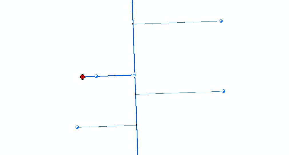
First, we will start with a traditional view of water distribution within a geometric network. This image should look familiar to GIS users that interact with water distribution data in a GIS, while individual corporations may choose a different set of symbols to represent assets, the data build is generally consistent.
Below we see a water main with 3 service leads, a hydrant lead, and hydrant with various types of fittings and valves present as well. Since this is geometric network-based data, we have all the points and lines connected (snapped) to one another, allowing us to perform flow-based analysis such as a water main break isolation trace to determine which valves need to be closed. Regardless of aesthetics such as symbols and colors, this is a very standard low fidelity data build. As we pan across this type of data build, we will continue to see assets captured in the same spirit of direct linear connectivity.
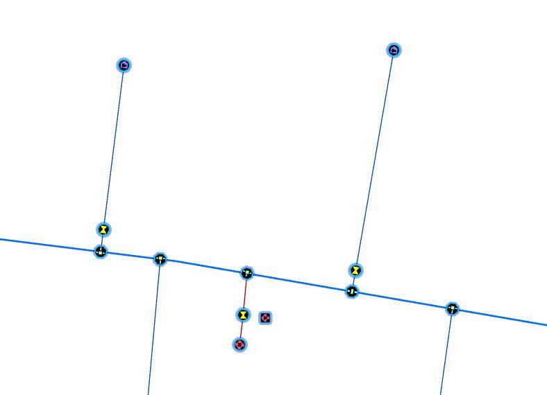
Comparing this to a similar data build in the utility network data model, we see some similarities but also certain components that are constructed differently, incorporating the new high-fidelity approach. One obvious difference is ESRI’s new high-quality web-based symbol library. We now have access to a more sophisticated set of asset icons that render very nicely in a web enabled environment. Much of the data build looks similar to our previous low fidelity example and we see water mains connecting to service leads via fittings and valves placed accordingly, but we also have a fire hydrant, and this appears different.
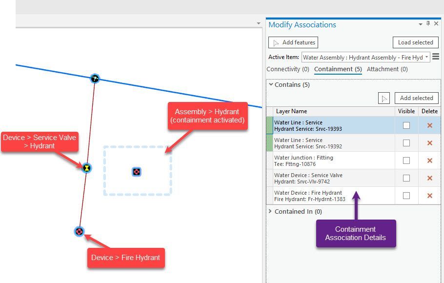
If we zoom in and examine this hydrant, we see a very different data build from what most people are used to. On this hydrant build we encounter a containment association; a fire hydrant point (layer = device) located geographically, but to the side we also have a hydrant assembly point (layer = assembly). We can use our utility network toolbar in ArcGIS Pro to ‘enter containment’ and learn more about this point. When we activate containment on this point, we know it is active by the dashed square outline around the assembly point (shown below). The containment properties for this point feature can be accessed using the modify associations tool, which shows the following assets related through association:
- 2 water service lines (both sides of the service valve
- One tee fitting
- One hydrant service valve
- One hydrant device
By using containment association for this asset build we have associated multiple assets of the fire hydrant build to the assembly point. These assets and their attributes are all accessible for analysis from a single assembly point using containment association.
Recall from our utility network introduction article that within a domain network we only have four layers to capture assets in. In our hydrant example we are using the layers: device, assembly and line. The GIS editor for this high-fidelity data will be responsible to create and maintain the assets, the assembly, and the assembly containment association.
Let's examine another, more ambitious, data build that uses containment association – a pumping station. A pumping station is one of the most complex facilities in a water distribution system and is used to perform a variety of functions based on the location and parameters of a given system. In our example below, we see another advancement in utility network in that polygons are now part of this network; this was not possible under geometric networks. Once again, we can ‘enter containment’ in our utility network toolbar and select the polygon (structure boundary > water pump station boundary). We know that containment is active by the dashed rectangle (containment can only be active on one object at a time) and by using the modify associations tool we see that there are 16 assets participating in this containment association.
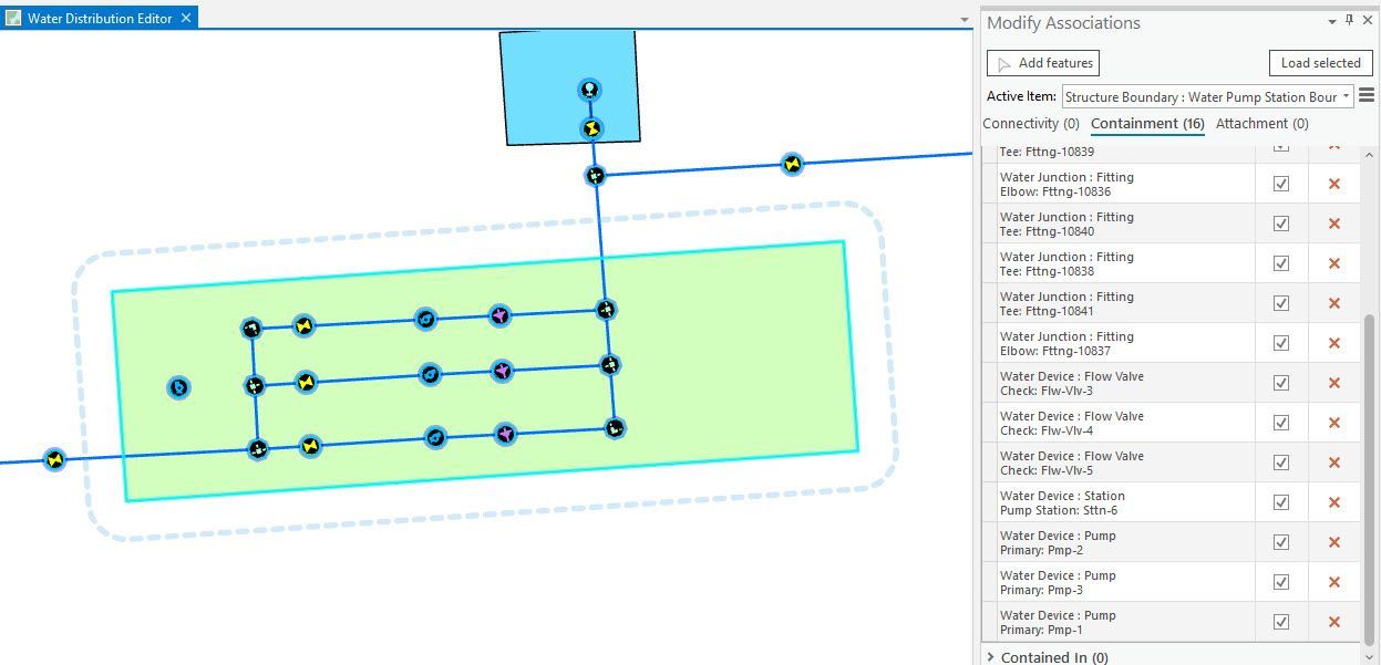
Once again, we can see how a significant amount of information is accessible through this containment association- a variety of fittings, pumps and valves are all associated to this site. The data editor will be responsible to create, edit, and maintain the assets as well as their role in the containment association.
Our final example will illustrate connectivity associations and how they can be used in conjunction with containment associations. One of the challenges with geometric networks was how to incorporate account-based data into a network that requires linear connectivity. While meters are easily incorporated to this type of network, since it is a physical asset, the account details are not a type of physical asset and multiple accounts may be associated with a single meter. We have seen many approaches to this challenge over the years. Now we can use associations to help tackle this challenge.
Below we see a metering station, the meter station point is selected, containment is activated and the modify associations pane is active. In it we see that there are 33 assets in the containment association. One type of asset participating in this association are water meters.
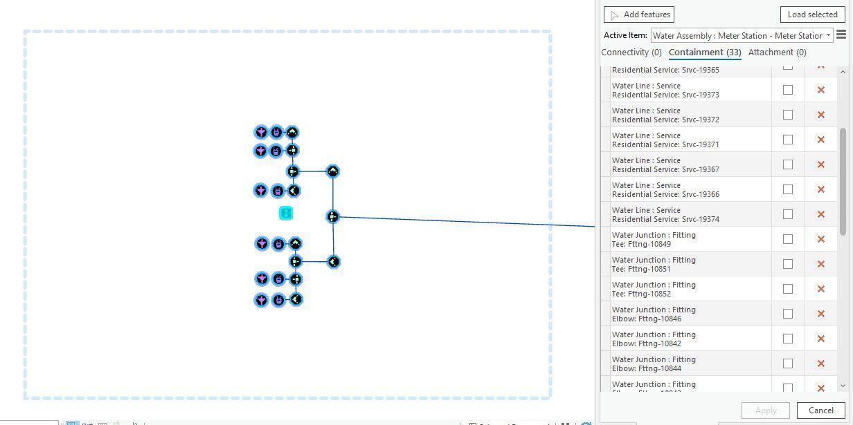
If we zoom out slightly, we can also see an additional series of points in proximity that appears unconnected to these assets shown in containment. These are residential service connections and represent an account where we would store account numbers. Some users familiar with geometric networks may interact with a similar build of data for account information, perhaps joined to the meter in a tabular relationship or perhaps even pseudo lines that establish the linear connectivity we discussed earlier.
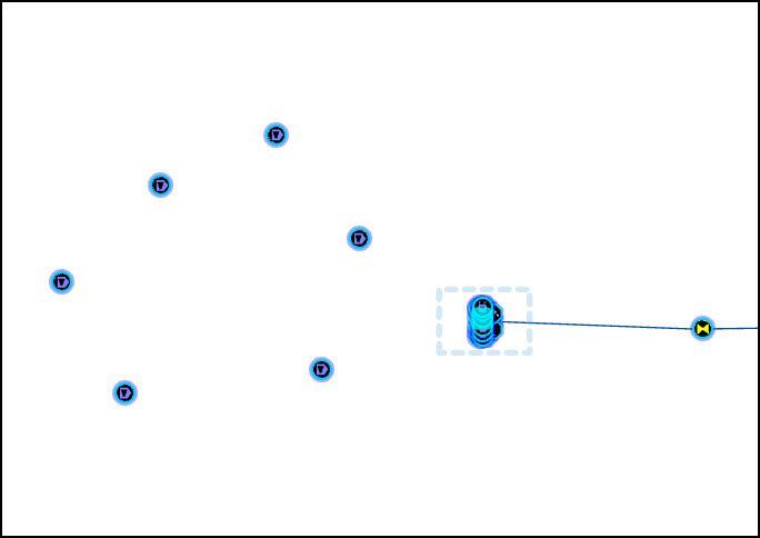
If we go back to our utility network tool bar in ArcGIS Pro and toggle on our view associations tool, we see that these account points are actually connected to certain meters via connectivity association - another type of association that we discussed previously.
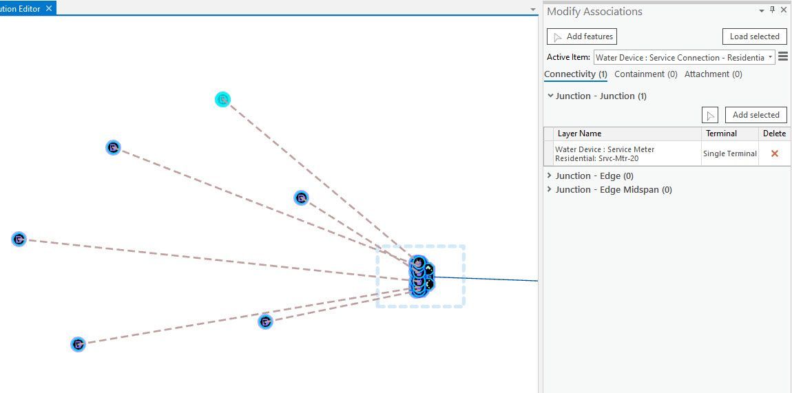
By participating in connectivity association these account points participate in the network and can therefore participate in network tracing type of analysis. For example, if we were to build a trace whereby a control valve was closed and blocked resource flow to this site, not only will our trace return the assets affected by this valve closure it will also include these accounts. In our example below you can see the account point is selected and the modify association pane shows us which meter point is connected and the type of association (connectivity).
Acorn Information Solutions launched its MonARC Data Migration platform to help corporations implement, or migrate to, a Utility Network. AIS has decades of experience in creating and administering municipal and utilities based Geometric Networks combined with knowledge and experience in Utility Network migrations.
About the Author
Craig Martin is Acorn’s Municipal and GIS Manager and has over 25 years of experience in the field of GIS. Craig has extensive experience in data modeling, data capture, administration, solutions architecture, and smart data networks in a variety of engineering disciplines. Connect with one of our experts at info@acorninfosolutions.ca